ITAPS
Petascale Technologies
Research | Partition Improvement | Predictive Load Balance | Communication Libraries | MapReduce Experiments | Scaling Results
Partition Improvement
The ability to scale implicit finite element and other implicit mesh-based computations on massively parallel computers requires ensuring both the system formulation and solution are effectively load balanced. Graph-based partitioners are well known to produce a partitioning of the mesh into parts that are well balanced, in terms of the specified partition object type, while also minimizing inter-part communications. However, traditional graph-partitioners consider a single objective optimization subject to a single balance constraint.
In the case of mesh-based analysis, the defined graph nodes are often mesh regions. This selection does an excellent job of balancing the number of regions (elements) and therefore the workload for the construction of the part-level finite element system. However, the workload balance for the iterative solution (e.g. matrix vector product and vector norms) of the resulting system is proportional to the number of mesh vertices. Since mesh vertices are not the objects in the original partitioning, the balance may not be optimal, particularly when the numbers of mesh entities per part is relatively low (e.g., a few thousand).
We are developing two multiple compute-object based partitioning improvement algorithms to reduce the vertex imbalance thereby improving the overall balance of two mesh entities as required by a scalable implicit solve. They are referred to as local iterative inter-part boundary modification (LIIPBMod) and heavy part split (HPS).
The LIIPBMod Algorithm. LIIPBMod locally migrates small numbers of mesh regions from parts that are relatively heavily loaded with respect to mesh vertices to neighboring parts which are relatively lightly loaded with respect to mesh entities. On the heavily loaded part, the mesh vertices on the part boundary are traversed and the ones bounding a small number of elements are identified. If the neighboring part is lightly loaded, the whole “cavity” (all the adjacent elements of the picked vertex) is migrated to the neighboring part. By this minor inter-part boundary adjustment, the vertex imbalance is improved while only modestly perturbing the good element balance. This procedure may need to be repeated for several iterations to achieve desired vertex balance.
The HPS Algorithm, Our studies of the mesh partitions given by a graph-based partitioner show that the percentage of heavily loaded parts (more than 10% imbalance) is usually less than 1%. The idea of HPS is that, if the desired number of parts is numP, first distribute the mesh to 99%*numP parts by a graph-based
partitioner and leave the other 1%*numP parts empty. Then, select the 1%*numP parts with the highest vertex load and split them into two parts (i.e. migrate roughly half of the mesh entities from them to one of the empty parts). The splitting makes the heavily loaded parts become lightly loaded. Since the peak of the imbalance determines the scalability, HPS lowers the peak and hence improves the performance.
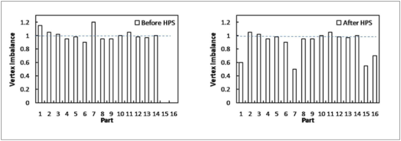
Figure: Vertex imbalance before and after HPS for a 16 part example. The partitions on parts 1 and 7 are split and given to parts 15 and 16 to improve overall performance.
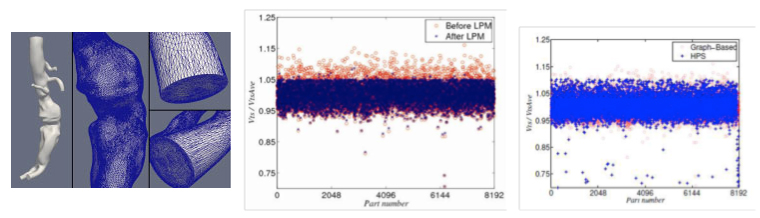
Figure: Vertex imbalance before and after applying LIIPBMod and HPS to a 16.7M element anisotropically adapted mesh used in the simulation of an abdominal aorta aneurism (left image). The two graphs (center for LIIPBmod and right graph for HPS) indicate the average number of vertices per part divided by the average per part before (red dots) and after (blue dots) application of the algorithms. Note in both cases the spikes (red dots in the upper parts of the graphs) that reduce scalability are dramatically lowered after the algorithms have been applied.
Using these techniques on a 1 billion element element mesh, we are able to achieve 88% efficiency on a strong scaling study using the PHASTA unstructured mesh element solver on Intrepid (BG/P system).
# of cores |
Rgn imb |
Vtx imb |
Time (s) |
Scaling |
16k |
2.03% |
7.13% |
222.02 |
1 |
32k |
1.72% |
8.11% |
112.43 |
0.987 |
64k |
1.6% |
11.18% |
57.09 |
0.972 |
128k |
5.49% |
17.85% |
31.35 |
0.885 |
Table 1. One billion element anisotropic mesh on Intrepid Blue Gene/P